Code Gradient Descent From Scratch

How to program gradient descent from scratch in python. For that time you fumbled in the interview.

Physical and chemical gradients within the soil largely impact the growth and microclimate of rice paddies

Motivation

This is it. You’ve networked your way through the door by sending approximately 10 LinkedIn messages to perfect strangers and charming the recruiter through that 30-minute phone call summarizing your entire adult professional life. They’ve sent you…dun dun dun….the assignment. 4 hours they say. Just 4 short hours. “4 hours,” you think to yourself “piece of cake”. The email comes along with the link to a google doc of instructions. “Just 2 prompts” you think again, “No problem at all. Bet I’ll have time to spare.” You open the assignment. There. Sprawled across the first google sheet reads “Please minimize this unknown function”. Your brain goes dark and you contemplate whether you could pass a fifth-grade math test.

The Prompt

Alright so let’s take a fresh look at what this interviewer is trying to get you to do:

Given: You pull the function from something like a pickle file, so you only know the inputs (which you specify) and the output (given by the function).

Problem: Find the inputs which minimize the output of this function by computing the gradient at each given point. For example we’ll use f(x1,x2)=y

Background

This is gradient descent. It’s just broken down into the components. You know it. You’ve learned it before. There are so many articles on gradient descent that I can’t justify why writing about it extensively here would provide value. A few good resources are this article for quick review and the classic Andrew Ng course for everything you’ve ever wanted to know. For now, I’ll remind you of the basics required to complete this challenge.

What is a gradient?

The book definition: a gradient is the magnitude and direction of change from one point to another.

The practical definition: Before I switched to data science I studied engineering, so my best examples of gradients are rooted in mechanics and fluid dynamics. Hopefully, this analogy will be absolutely perfect for one person, and tolerable for everyone else. Imagine a lake. Pretty calm typically.

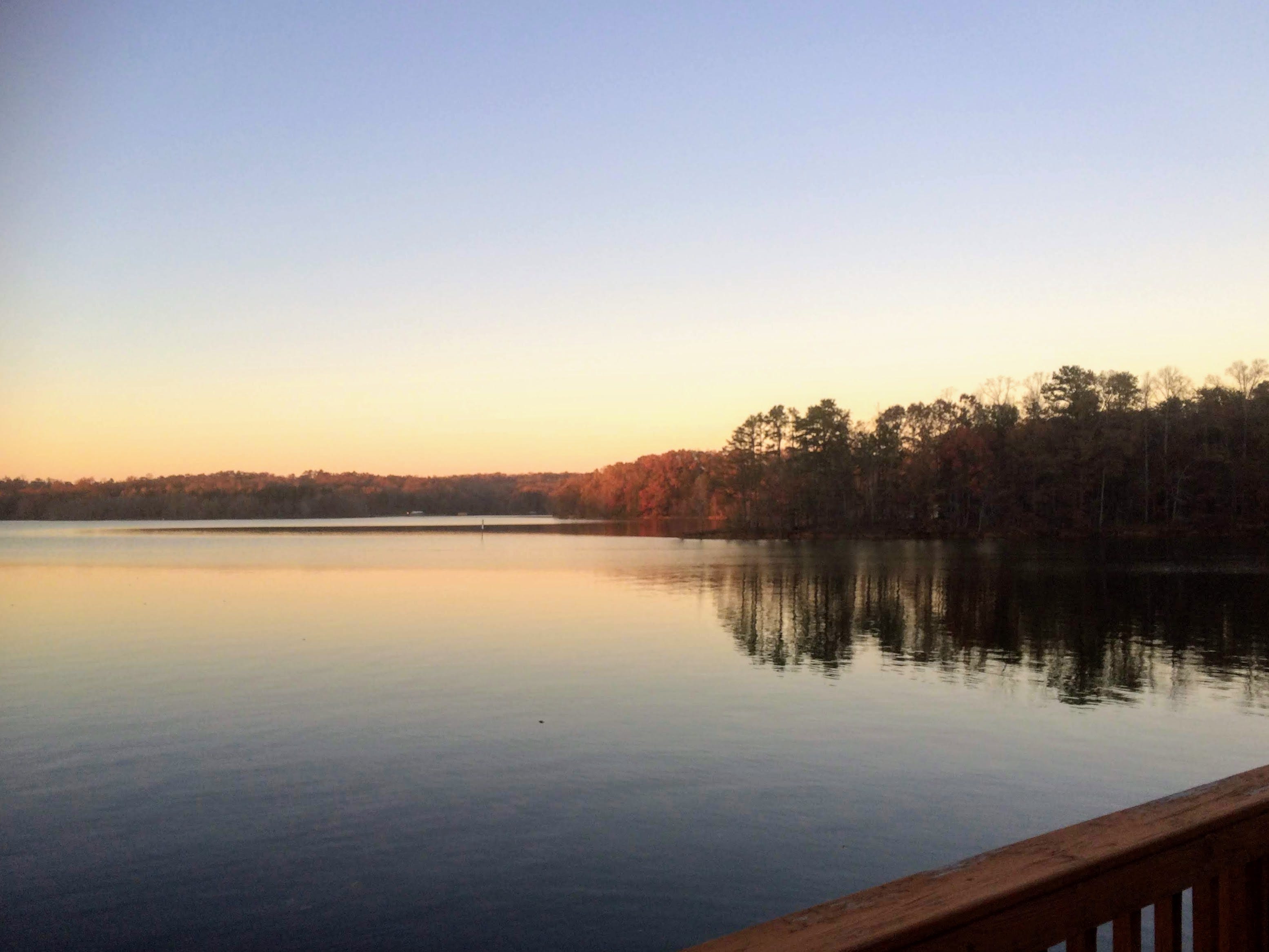Photo by Author

Ok, now a boat comes through pulling a phenomenal slalom skier. Does the water still have the same current throughout?

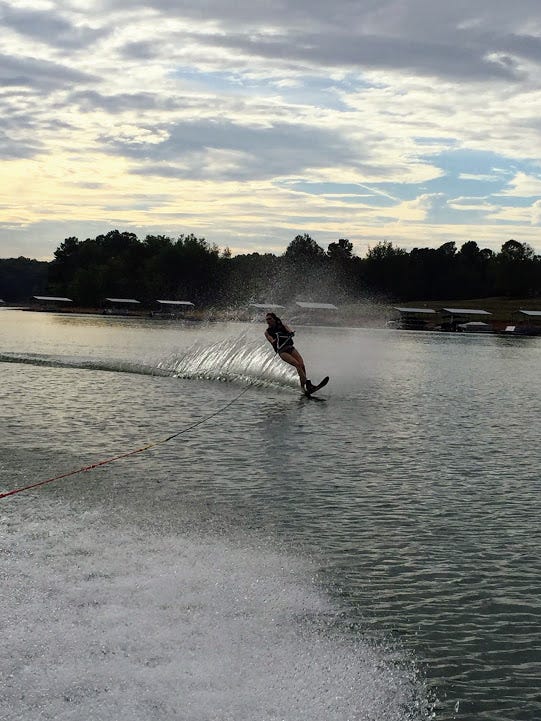Photo by Author

The water likely doesn’t have the same speed and direction across the entire surface anymore right? How could we represent the speed and direction of the water on different parts of this lake? Well, mechanical physics would tell you to use a velocity vector. Like so:

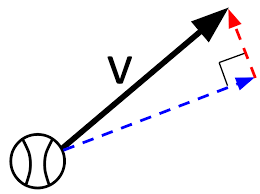Image by Khan Academy

This represents one gradient. Velocity is the change in distance (in a particular direction) from one point to another with respect to time. Start combining these gradients and we get something that looks like this:

Image by David Cheneler via ResearchGate

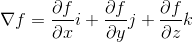
The math definition: A gradient is the slope of the line tangent to the curve at whatever point you are assessing. This means a gradient is the sum of the partial derivative components representing that function at that point. Which brings us to something like this:

What are we descending and why?

In machine learning, you are typically trying to find some relationship between a predictor and a series of features. To converge you optimize a cost function for the lowest amount of error. The way you optimize this is by taking steps in the direction of the lowest error and returning the gradient vector that corresponds. Once you reach a threshold minimum your gradient vector reveals the coefficients which optimize this cost function.

Put another way…perhaps you’ve seen this before:

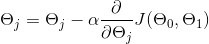
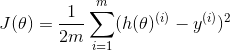
This is the equation for gradient descent assuming you have some known cost function J(theta) and learning rate (alpha). A common cost function for linear regression, for instance, is the sum of squared error:

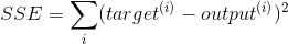
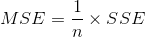
In this equation, we are computing squared error via our target (y_pred) and our output (y_actual). Next, we compute the mean of squared errors by diving by our number of observations (n). To combine both of our equations here in the case of linear regression let’s represent our cost function in terms of squared error.

Here we are using m instead of n to indicate the number of observations in this step, and we are dividing by 2 simply to make differentiation easier when we compute the gradients. h(theta) represents the target (y_pred) and y represents output (y_actual). Plugging back into the first equation you end up with something like the following:

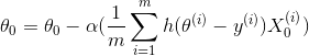
Here alpha represents the learning rate as in the first equation, but we have already solved the partial derivative for the gradient.

Let’s move back to the interview question where the (cost) function is unknown. We don’t have the luxury of computing partial derivatives. Therefore, we’ll have to use a guess and check method of finding the maximum gradient. Instead of computing the gradient, I will simply specify a step size (as you will see below). I will use that step size to check each gradient around the current point.

This is pretty brute force, but I would presume that your interviewer is testing whether or not you can dive under the hood of your algorithmic vehicle and conduct a bit of manual maintenance.

Coding the Solution

Alright, let’s get down to it. I made two functions to solve this problem. The first function will simply compute the maximum gradient given x = (x1, x2). I’m going to presume there are only 2 features (x1,x2) as defined by the prompt. The second function will use that first function to minimize your unknown (given) function f(x1,x2) = y by following gradients in the first function. Starting with the first function we have:

def gradient(func,x):
	# func = the unknown function you are given
	# x = (x1,x2) 
    # Define step size and current y
    step = 1
    y = func(x)
    
    # Check all points around x,y for the largest difference (gradient magnitude)
    # Neg points 
    x_neg = (x[0] - step, x[1]-step)
    y_neg = func(x_neg)
    diff_neg = y - y_neg
    # Pos points
    x_pos = (x[0] + step, x[1]+step)
    y_pos = func(x_pos)
    diff_pos = y - y_pos
    # Pos Neg points 
    x_pn = (x[0]+step, x[1]-step)
    y_pn = func(x_pn)
    diff_pn = y - y_pn
    # Neg Pos points
    x_np = (x[0]-step, x[1]+step)
    y_np = func(x_np)
    diff_np = y - y_np
    diff = [diff_neg, diff_pos, diff_pn, diff_np]
    
    # Compare diffs
    if max(diff) == diff_neg:
        # Returning the magnitude and direction of the gradient
        grad = (x_neg, diff_neg)
    elif max(diff)==diff_pos:
        grad = (x_pos, diff_pos)
    elif max(diff)==diff_pn:
        grad = (x_pn, diff_pn)
    else:
        grad = (x_np, diff_np)
    return grad

What’s happening here is that I’m grabbing the difference between every point around my given point (x1,x2) and my given point + the step size I instantiated (here it is 1). Then I’ll find the maximum of these 4 differences and return the direction (x1+step,x2+step) and magnitude (difference) associated.

Let’s take a look at the minimizing function:

def minimize(func, debug=False):
	# func = the unknown function you are given
	# Define where you want to start minimizing from (x)
	# Define the threshold difference to stop at (closest to minimum point)
    x = (600,600)
    diff = 99999999
    stop = 0.00005
    
    # Until you reach threshold (stop) --> minimize
    while abs(diff) > stop:
        grad = gradient(func,x)
        diff = grad[1]
        x = grad[0]
        if debug:
            print(grad[0],grad[1])
    return print("Minimum Point: (%.2f,%.2f)"%(grad[0][0], grad[0][1]))

Here I’m stepping through my gradients using the returned maximum from my gradient function to rerun the loop every time. Once I’ve reached a stopping difference that is close to zero I return the coordinates (x1,x2) of the function at that point. I’d also recommend visualizing this (if possible) to get a feel for your solution. My example looked like this:

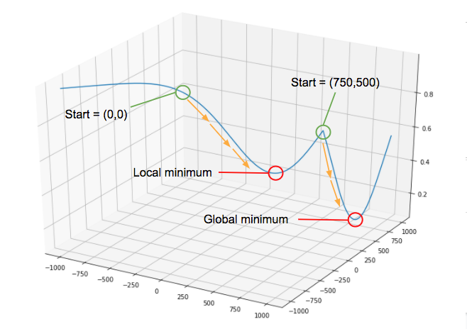Image by Author

As you can see there is a local minimum in addition to the global minimum. If I only initialize the minimize() function at (0,0) I’ll get stuck in the local minimum. I got around this problem by initializing the script at randomly different starting points to ensure a true minimum. Once the minimize() function starts at ~(750,500) I’m able to find the global minimum. Momentum is a popular concept in neural networks that accomplishes this task without having to initialize at random points (as you can imagine with 100+ features this could become tedious). It’s a bit out of scope for this post, but something to look into for scalable ways of reaching the global minimum.

In Conclusion

Some form of this problem is pretty typical for a machine learning interview. I also think it’s a fun puzzle for showing some basic python chops as you don’t need any fancy packages for this. A few references I used to approach this problem are below and I wish you the best of luck in future interviewing endeavors. May you descend gradients with grace.

References

• Wikipedia on Gradients

• Gradient Descent in Python

• Gradient Descent Math

• Gradient Descent Equations

Originally published at https://brittanybowers.com on April 1, 2020.